Neural Networks

This is a learning note related to the Neural Networks (NNs).

1. Basics

   • The chain rule for computing a composition of two functions:

     \[\nonumber \frac{\partial f(g(x))}{\partial x} = f'(g(x))g'(x)\]

     And it can be extended as

     \[\nonumber \frac{\partial f(g_1(x), g_2(x), ..., g_n(x))}{\partial x} = \sum_{i=1}^n \frac{f(g_1(x), ..., g_n(x))}{\partial g_i(x)} \frac{\partial g_i(x)}{\partial x}\]

​

1. Neural Networks

   The learning process of NNs is using data to adapt (train) the parameters (weights) of a mathematical model.

   • Notations:

     • Input $x_1, …, x_d$ is collected in vector $\boldsymbol{x}\in \mathbb{R}^d$ ,

     • NN can be described by a weighted directed graph

       • Integers $V = {0,1,2…}$ are the names of neurons (nodes/ vertices in the graph).

         given $d$ input neurons, $K$ output neurons, $M$ hidden neurons:

         \[\nonumber V = \{0\} \cup V_{\text{input}} \cup V_{\text{hidden}} \cup V_{\text{output}} = \{0,1,2..., d+M+K\}\]

         Where $V_{\text{input}} = {0,…,d}$, $V_{\text{hidden}} = {d+1, …, d+M}$, $V_{\text{output}} = {d+M+1, …, d+M+K}$

       • Edges A are connections between neurons. $(j,i) \in A$ is an edge from neuron $j$ to neuron $i$ is described by weight $w_{ij}$. All weights are collected in weight vector $\boldsymbol{w}$.

     • “Integration”: computing weighted sum with bias (threshold, offset) parameter $w_{i0} \in \mathbb{R}$

       \[\nonumber a_i = \sum_{j=1}^d w_{ij}x_j + w_{i0}\]

     • Activation function of neuron $i$ is denoted as $h_i$

       • $h_i(a) = a \text{ for $i \in {0} \cup V_{\text{input}}$}$
       • Typically $h_i \neq h_j \text{ for $i \in V_{\text{hidden}} \text{ and } j \in V_{\text{output}}$}$

     • The output of neuron $i$ is denoted as $z_i(\boldsymbol{x})$

       \[\nonumber z_i = h_i(a_i) = h(\sum_{j=1}^d w_{ij}x_j + w_{i0})\]
       • $z_0(\cdot) = 1$
       • $z_i(\cdot) = x_i \text{ for } i \in V_{\text{input}}$

     • The output of the network:

       \[\nonumber f(\boldsymbol{x}; \boldsymbol{w}) = \pmatrix{z_{M+d+1} \\ z_{M+d+2} \\ ... \\ z_{M+d+K}} = \pmatrix{\hat{y_1} \\ \hat{y_2} \\ ... \\ \hat{y_K}}\]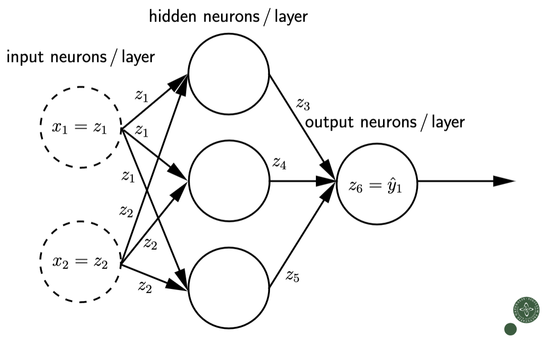

       

       Fig 1. NN -- weighted directed graph

   • Loss Function and Gradient

     Here we define $L$ represents loss function, sum of the square errors for $N$ samples ($N$ pairs of input)is below,

     \[\nonumber E = \frac{1}{2}\sum^N_{n=1}\Vert f(\boldsymbol{x}\boldsymbol{; w}) - \boldsymbol{y}\Vert^2 = L\left(f(\boldsymbol{x;w}), \boldsymbol{y}\right)\]

     The gradient of $\boldsymbol{w}$ is the transpose of partial direvitive of $E$ with respect to $\boldsymbol{w}$ (The reason why it is transpose is that the gradient is normally column vector), namely:

     \[\nonumber \nabla_w E = (D_wE)^\text{T} = (D L \cdot D_w f)^\text{T}\]

     Where

     \[\nonumber DL = \frac{\partial L}{\partial f} \\ D_wf = \frac{\partial f}{\partial w} = \pmatrix{\frac{\partial f^1}{\partial w^1} & ... & \frac{\partial f^1}{\partial w ^M}\\... & ... & ... \\ \frac{\partial f^K}{\partial w^1} & ... & \frac{\partial f^K}{\partial w^M}}, \text{ Jacobian Matrix}\]

   • Back Propagation

     We have know how to compute the gradient and we can choose different optimizer to apply different strategy to update the weights. But why the update process is called back propagation?

     Go back to the previous chapter, the computation of gradient can be written as

     \[\nonumber \begin{aligned} f(\boldsymbol{x}, \boldsymbol{w}) &= \boldsymbol{h}^N (\boldsymbol{w}^N \boldsymbol{h}^{N-1}(\boldsymbol{w}^{N-1} ... \boldsymbol{h}^1 (\boldsymbol{w}^1 \boldsymbol{x}))) \\ D_wf = \frac{\partial f}{\partial \boldsymbol{w}} &= D\boldsymbol{h}^N D\boldsymbol{w}^N D\boldsymbol{h}^{N-1} D\boldsymbol{w}^{N-1} ... D\boldsymbol{h}^1 D\boldsymbol{w}^1 \\ \nabla_w E &= (D_wE)^\text{T} = (D_wf)^{\text{T}}(DL)^{\text{T}} \\ &= (D\boldsymbol{w}^1)^{\text{T}}(D\boldsymbol{h}^1)^{\text{T}}...(D\boldsymbol{w}^N)^{\text{T}}(D\boldsymbol{h}^N)^{\text{T}}(DL)^{\text{T}} \end{aligned}\]

     where the superscript numbers $1, …, N$ represent the corresponding layers.

     As the gradient for weights at the last layer are always need to be computed than that at previous layers, so the process of updating is called back propagration (computes the gradient from the back to the front, thus updating the weights from the back to the front).